Methodology
Table of Contents
Overview
The RUM Archive datasets contain aggregated Real User Monitoring (RUM) data from one or more websites.
Each dataset in the RUM Archive publishes aggregated RUM data to public Google BigQuery tables.
There are two types of tables within the RUM Archive:
- Page Loads: Browser page load experiences
- Resources: Third party resource fetches
The documentation on this page describes how this RUM data is aggregated, exported and made available for querying.
Aggregation
All data published to the RUM Archive is sanitized and aggregated.
The goal of aggregation is twofold:
- To protect the privacy of individuals who visit a website
- To reduce the amount of data that needs to be stored in the tables, so that vast quantities of data can be represented
In order to generate queryable aggregated data, each RUM Archive table shares a common pattern in the columns it contains:
- Multiple Dimensions that describe the aggregate data, such as date, browser, geographic region, or protocol
- Each row represents a unique tuple of those dimensions
- A Count of the number of datapoints that match that unique tuple
- Timers or Metrics that are aggregated into Histograms and other statistics like Avg or SumLn
With the data exported in this format, anyone wanting to combine, aggregate, slice, filter or group by any of the available dimensions can also calculate statistics about the Timers and Metrics for that group of data:
- By using the Histogram columns, queries can calculate approximate percentiles of the data (from 0th to 100th).
- By using the Avg columns and Count columns, queries can calculate the average of data.
- By using the SumLn and Count columns, queries can calculate the geometric mean of data.
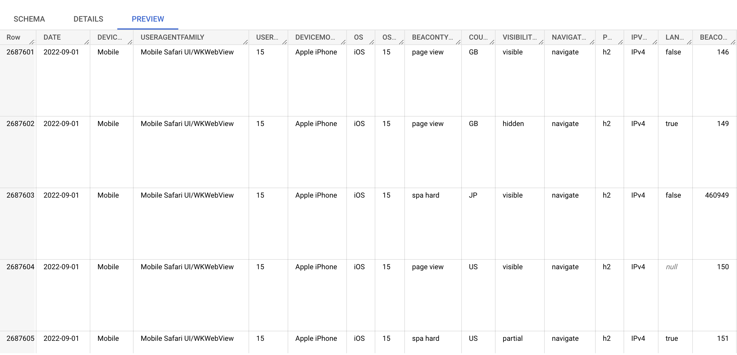
Here's an example screenshot of a few rows of the Dimension and Count columns. Each row has a distinct set (tuple) of columns, and a Count of how many experiences matched those tuples:
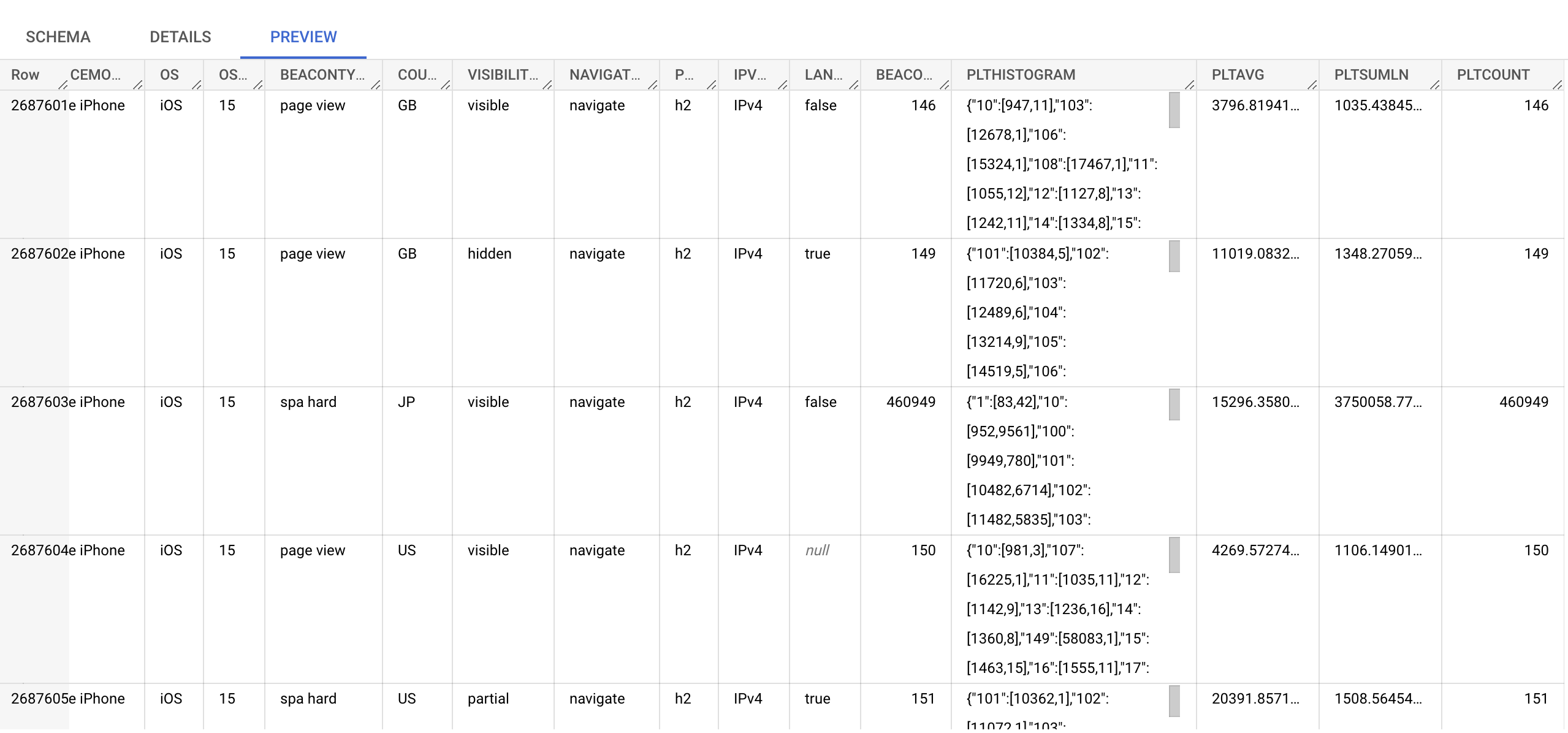
Looking at a few further columns for the same rows, you can see the Page Load Time columns (PLT*) show a Histogram, Avg, SumLn and Count of those aggregated datapoints.
Minimum Count Threshold
Some datasets may have a Minimum Count Threshold for aggregated data. For example, the mPulse dataset has a Minimum Count Threshold for the Page Loads table of 5, so all tuples in the exported data that aren't represented by at least 5 unique hits will be discarded.
Other datasets may have a Minimum Count Threshold of 1, so all available data is represented in the dataset. For example, the Akamai Employee Individual Datasets contain all of the page load events for each day.
The downside of applying a Minimum Count Threshold is that outliers, by definition, will be discarded and not represented in the queryable dataset.
Discarding outliers will affect the accuracy of queries. For example, in the mPulse dataset, we estimate that discarding any tuples with less than 5 hits could affect 50th percentile (median) calculations by around 2.9% and 95th percentile calculations by 7%. Please take this into consideration when querying the data.
Histogram Bucketing
RUM Archive tables contain several Histogram columns, one for each timer or metric that is aggregated.
These Histogram columns are used to calculate approximate percentiles of the data.
Each Histogram is a frequency distribution of datapoints for that timer/metric, according to the bucket widths described below.
All Histograms contain 152 buckets:
- Zero values: 1 bucket (bucket 0)
- High precision: 100 buckets (buckets 1-100)
- Low precision: 50 buckets (buckets 101-150)
- Anything higher than the Max: 1 bucket (bucket 151)
High precision buckets are on the low end of the expected value range, and represent values where the impact of the metric changing is the highest. For example, Page Load Time's High Precision buckets start at 0 and go to 10,000ms in 100 equally-sized 100ms buckets.
Low precision buckets extend to the numbers beyond the High Max, using buckets 10x the width of the High Width. For example, Page Load Time's Low Precision buckets start at 10,001ms and extend to 60,000ms in 50 equally-sized 1,000ms buckets.
Having both High precision and Low precision buckets allows us to represent data from a large range of possible values while still providing high precision to the values that matter most (on the low end of the range).
By combining all of the Histograms for columns matching a query, and running the fast histogram algorithm on the combined Histograms, one can calculate the approximate percentile for any timer/metric.
Histogram Format
Histograms are stored in a JSON object format.
Each key represents the bucket number, and the value is an array of two values:
[0]is the mean of values in that bucket[1]is the count of values in that bucket
An example Page Load Histogram for a single row may look like this:
{
    "102": [11679, 1],
    "103": [12803, 1],
    "106": [15876, 2],
    "113": [22532, 1],
    "117": [26026, 1]
}
In the above example, there are 6 values:
- Bucket # 102, which represents data between 11,000ms and 11,999ms has a single value, of 11,679ms.
- Bucket # 106, which represents data between 15,000ms and 15,999ms has a 2 values, with a mean of 15,876ms.
Page Loads Histogram Buckets
Page Loads have following bucket histogram definitions:
| Metric | Column Name | High Width (ms) | High Min (ms) | High Max (ms) | Low Width (ms) | Low Min (ms) | Low Max (ms) |
|---|---|---|---|---|---|---|---|
| Page Load Time | PLTHISTOGRAM |
100 | 0 | 10,000 | 1,000 | 10,001 | 60,000 |
| DNS | DNSHISTOGRAM |
10 | 0 | 1,000 | 100 | 1,001 | 6,000 |
| TCP | TCPHISTOGRAM |
10 | 0 | 1,000 | 100 | 1,001 | 6,000 |
| TLS | TLSHISTOGRAM |
10 | 0 | 1,000 | 100 | 1,001 | 6,000 |
| Time to First Byte | TTFBHISTOGRAM |
10 | 0 | 1,000 | 100 | 1,001 | 6,000 |
| First Contentful Paint | FCPHISTOGRAM |
100 | 0 | 10,000 | 1,000 | 10,001 | 60,000 |
| Largest Contentful Paint | LCPHISTOGRAM |
100 | 0 | 10,000 | 1,000 | 10,001 | 60,000 |
| Round Trip Time | RTTHISTOGRAM |
10 | 0 | 1,000 | 100 | 1,001 | 6,000 |
| Rage Clicks 1 | RAGECLICKSHISTOGRAM |
1 | 0 | 100 | 10 | 101 | 600 |
| Cumulative Layout Shift (*1000) | CLSHISTOGRAM |
10 | 0 | 1,000 | 100 | 1,001 | 6,000 |
| First Input Delay | FIDHISTOGRAM |
10 | 0 | 1,000 | 100 | 1,001 | 6,000 |
| Interaction to Next Paint | INPHISTOGRAM |
10 | 0 | 1,000 | 100 | 1,001 | 6,000 |
| Total Blocking Time | TBTHISTOGRAM |
100 | 0 | 10,000 | 1,000 | 10,001 | 60,000 |
| Time to Interactive | TTIHISTOGRAM |
100 | 0 | 10,000 | 1,000 | 10,001 | 60,000 |
| Redirect | REDIRECTHISTOGRAM |
10 | 0 | 1,000 | 100 | 1,001 | 6,000 |
| Unattributed Navigation Overhead | UNOHISTOGRAM |
10 | 0 | 1,000 | 100 | 1,001 | 6,000 |
rageClicksHistogramwas changed on 2023-01-01, see the blog post for details.
Third-Party Resource Histogram Buckets
Third-Party Resource fetches have following bucket histogram definitions:
| Metric | Column Name | High Width (ms/b) | High Min (ms/b) | High Max (ms/b) | Low Width (ms/b) | Low Min (ms/b) | Low Max (ms/b) |
|---|---|---|---|---|---|---|---|
| Total Time | TOTALHISTOGRAM |
10 | 0 | 1,000 | 100 | 1,001 | 6,000 |
| DNS Time | DNSHISTOGRAM |
10 | 0 | 1,000 | 100 | 1,001 | 6,000 |
| TCP Time | TCPHISTOGRAM |
10 | 0 | 1,000 | 100 | 1,001 | 6,000 |
| TLS Time | TLSHISTOGRAM |
10 | 0 | 1,000 | 100 | 1,001 | 6,000 |
| Request Time | REQUESTHISTOGRAM |
10 | 0 | 1,000 | 100 | 1,001 | 6,000 |
| Response Time | RESPONSEHISTOGRAM |
10 | 0 | 1,000 | 100 | 1,001 | 6,000 |
| Time to First Byte | TTFBHISTOGRAM |
10 | 0 | 1,000 | 100 | 1,001 | 6,000 |
| Download Time | DOWNLOADHISTOGRAM |
10 | 0 | 1,000 | 100 | 1,001 | 6,000 |
| Redirect Time | REDIRECTHISTOGRAM |
10 | 0 | 1,000 | 100 | 1,001 | 6,000 |
| Cached1 | CACHEDHISTOGRAM |
- | - | - | - | - | - |
| Encoded Body Size | ENCODEDSIZEHISTOGRAM |
1000 | 0 | 100,000 | 10,000 | 100,001 | 600,000 |
| Decoded Body Size | DECODEDSIZEHISTOGRAM |
1000 | 0 | 100,000 | 10,000 | 100,001 | 600,000 |
| Transfer Size | TRANSFERSIZEHISTOGRAM |
1000 | 0 | 100,000 | 10,000 | 100,001 | 600,000 |
cachedis boolean (either0or1)
Example Aggregation Queries
Generating data in this format can be done with standard SQL queries.
The exact SQL will depend on the schema of the source table, but the mPulse Dataset provides an example SQL query in the rum-archive Github repository.
Exporting
Once RUM Archive data has been generated, it should be exported to CSV or TSV and loaded into a Google BigQuery dataset.
The schemas for Page Loads and Resources tables are available in the rum-archive Github repository.
A convenient way to import TSV files into BigQuery is by uploading those files to a Google Cloud Storage bucket:
gsutil -m cp -Z -n *.tsv gs://%BUCKET%/Then executing a BigQuery LOAD DATA INTO command:
LOAD DATA INTO `%PROJECT%.%DATASET%.%PREFIX%_page_loads`
(
    SOURCE STRING,
    SITE STRING,
    DATE DATE,
    DEVICETYPE STRING,
    USERAGENTFAMILY STRING,
    USERAGENTVERSION STRING,
    DEVICEMODEL STRING,
    OS STRING,
    OSVERSION STRING,
    BEACONTYPE STRING,
    COUNTRY STRING,
    VISIBILITYSTATE STRING,
    NAVIGATIONTYPE STRING,
    PROTOCOL STRING,
    IPVERSION STRING,
    LANDINGPAGE BOOLEAN,
    BEACONS INTEGER,
    PLTHISTOGRAM STRING,
    PLTAVG FLOAT64,
    PLTSUMLN FLOAT64,
    PLTCOUNT INTEGER,
    DNSHISTOGRAM STRING,
    DNSAVG FLOAT64,
    DNSSUMLN FLOAT64,
    DNSCOUNT INTEGER,
    TCPHISTOGRAM STRING,
    TCPAVG FLOAT64,
    TCPSUMLN FLOAT64,
    TCPCOUNT INTEGER,
    TLSHISTOGRAM STRING,
    TLSAVG FLOAT64,
    TLSSUMLN FLOAT64,
    TLSCOUNT INTEGER,
    TTFBHISTOGRAM STRING,
    TTFBAVG FLOAT64,
    TTFBSUMLN FLOAT64,
    TTFBCOUNT INTEGER,
    FCPHISTOGRAM STRING,
    FCPAVG FLOAT64,
    FCPSUMLN FLOAT64,
    FCPCOUNT INTEGER,
    LCPHISTOGRAM STRING,
    LCPAVG FLOAT64,
    LCPSUMLN FLOAT64,
    LCPCOUNT INTEGER,
    RTTHISTOGRAM STRING,
    RTTAVG FLOAT64,
    RTTSUMLN FLOAT64,
    RTTCOUNT INTEGER,
    RAGECLICKSHISTOGRAM STRING,
    RAGECLICKSAVG FLOAT64,
    RAGECLICKSSUMLN FLOAT64,
    RAGECLICKSCOUNT INTEGER,
    CLSHISTOGRAM STRING,
    CLSAVG FLOAT64,
    CLSSUMLN FLOAT64,
    CLSCOUNT INTEGER,
    FIDHISTOGRAM STRING,
    FIDAVG FLOAT64,
    FIDSUMLN FLOAT64,
    FIDCOUNT INTEGER,
    TBTHISTOGRAM STRING,
    TBTAVG FLOAT64,
    TBTSUMLN FLOAT64,
    TBTCOUNT INTEGER,
    TTIHISTOGRAM STRING,
    TTIAVG FLOAT64,
    TTISUMLN FLOAT64,
    TTICOUNT INTEGER,
    REDIRECTHISTOGRAM STRING,
    REDIRECTAVG FLOAT64,
    REDIRECTSUMLN FLOAT64,
    REDIRECTCOUNT INTEGER,
    INPHISTOGRAM STRING,
    INPAVG FLOAT64,
    INPSUMLN FLOAT64,
    INPCOUNT INTEGER,
    UNOHISTOGRAM STRING,
    UNOAVG FLOAT64,
    UNOSUMLN FLOAT64,
    UNOCOUNT INTEGER
)
FROM FILES (
  format = 'CSV',
  field_delimiter = '\t',
  skip_leading_rows = 1,
  uris = ['gs://%BUCKET%/%FILE%.tsv']
)
;
Querying
Please see the Querying guide for how to query RUM Archive data.