Tips

Table of Contents

Data is sampled

All of the data in the RUM Archive is sampled.

The sampling rate may not be publicly disclosed, so BEACONS counts should only be used for relative weighting for that day.

The sampling rate may also change from day-to-day.

Counts should only be used for relative percentages

Since the data is sampled, absolute counts of BEACONS should only be used to compare data on the same DATE in a single dataset.

As the sampling rate may change from day-to-day, absolute count comparisons between days should not be used, only relative weights.

See the sample queries for examples of how to calculate relative weights.

Outliers are excluded

All of the data in the RUM Archive is sampled, aggregated, and only rows that meet the Minimum Count Threshold are included.

The downside of applying a Minimum Count Threshold is that outliers, by definition, will be discarded and not represented in the queryable dataset.

Discarding outliers will affect the accuracy of queries. For example, in the mPulse dataset, we estimate that discarding any tuples with less than 5 hits could affect 50th percentile (median) calculations by around 2.9% and 95th percentile calculations by 7%. Please take this into consideration when querying the data.

Zeroes matter (or not)

When querying Timer or Metric percentiles via the PERCENTILE_APPROX function, you will need to consider whether you want to include "zeros" in the percentile calculation.

For some Timers or Metrics, including zeros makes sense. For example, Cumulative Layout Shifts can have a value of 0.0, meaning no shifts happened. This is good and represents the ideal page load (no shifts). Including zeros will likely "shift" the PERCENTILE_APPROX calculation left (lower), by including those 0.0 page loads.

For other Timers like DNS, you may want to include or exclude zeros:

• If you're including zeros, you're including all page loads, even those that had no DNS lookup time (e.g. because DNS was cached). This would be done to understand the percentile of DNS time for all of your page visits, whether or not they had to do a DNS lookup.
• If you're not including zeros, you're only including page loads that had a DNS lookup (e.g. excluding those that had DNS cached). This would be done to understand the DNS lookup time when DNS had to be queried.

Data sets should not be compared

Each dataset comes from a different website (or set of websites), and is using a different collection, sampling and aggregation methodology.

As a result, datasets shouldn't be directly compared to one another unless you're looking at specific things that would not be affected by those caveats (such as understanding the relative weighting of Browser or Device Types seen).

Limiting BigQuery costs

RUM Archive tables are partitioned by DATE to aid in reducing query costs. When you're issuing a BigQuery query, you should almost always be using a DATE clause.

If you don't include a DATE clause, BigQuery may have to query the entire dataset. Some datasets could be 100s of GBs or larger.

For example, a single day in the mPulse RUM dataset should only be 3-5 GB. After a year of data, the entire mPulse dataset could be 2 TB or larger.

You may want to review what's available in the BigQuery free tier, to try to stay under those limits. With 1 TB of free queries, you should be able to run a few hundred queries against the mPulse dataset, when using a DATE filter.

BigQuery has an estimated query cost (in bytes) in the upper-right corner of the BigQuery console:

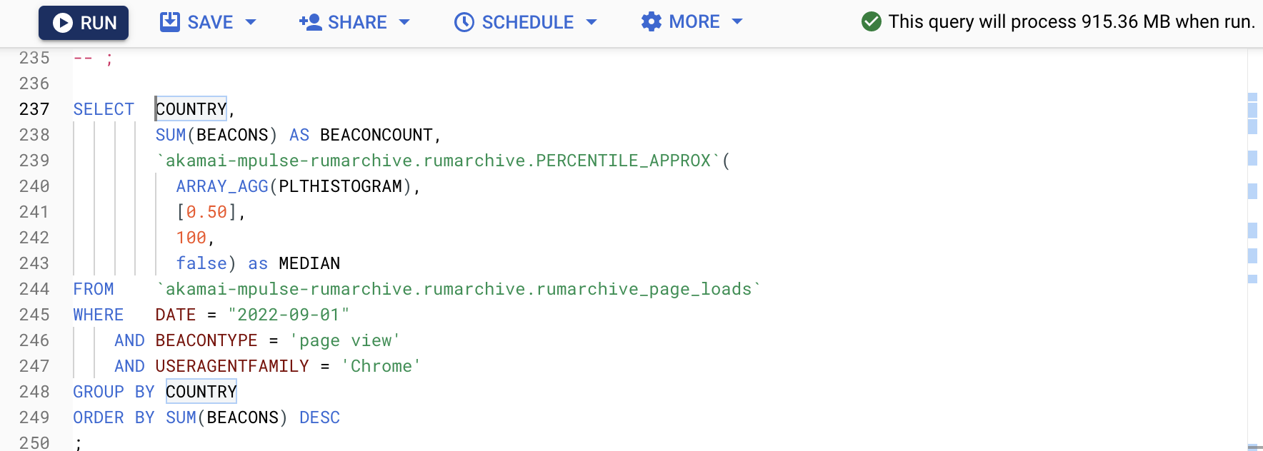
BigQuery UDF Out of Memory

When using the PERCENTILE_APPROX function, BigQuery may run out of memory:

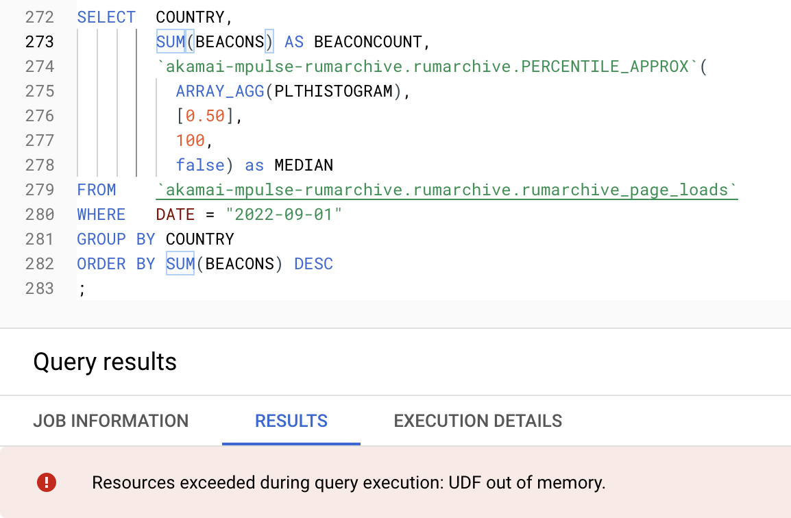
This is because PERCENTILE_APPROX is a JavaScript function (UDF), and it is combining histograms to calculate the approximate percentile for each output row. Sometimes, this work is too costly and BigQuery will run out of memory.

There are a few approaches to workaround this:

1. Utilize WHERE clauses to filter to a subset of the data (see this example)
2. Issue a sub-query against a high-cardinality dimension to break the dataset down first (see this example)
3. Export the data and run your own queries or aggregation

Not Every Timer is Available on Every Row

When generating aggregated data for BigQuery, the aggregation query contains a WHERE clause to only include rows that contain a Page Load Time.

Every timer, including Page Load Time, but also the other timers such as DNS or Largest Contentful Paint has 4 columns associated with it: *HISTOGRAM, *AVG, *SUMLN and *COUNT. The last column, *COUNT records how frequently that timer appeared for that row's tuples of data.

Since the aggregation is pivoted on Page Load Time being available, you can expect the BEACONS column (how many page loads the row represents) to equal the PLTCOUNT exactly. However, other timers may not be on every Page Load beacon. For example:

• Events like Rage Clicks may not always happen
• Timers like LCP may not have been recorded if the browser doesn't support the metric

As a result, for the non-PLT timers, you may see a *COUNT column lower than the BEACONS and PLTCOUNT columns.

As an example, if you see BEACONS == PLTCOUNT == 100 and DNSCOUNT == 10 that means that DNS data was only recorded on 10% of the page loads represented by that row.

Here are the timer counts and the percentage of beacons they were on, for one day's worth of data (2023-09-30):

Column	Count	% of Total
BEACONS	169,613,083	100.0%
PLTCOUNT	169,613,083	100.0%
DNSCOUNT	169,228,821	99.8%
TCPCOUNT	169,225,189	99.8%
TLSCOUNT	169,212,909	99.8%
TTFBCOUNT	169,226,039	99.8%
FCPCOUNT	105,779,526	62.4%
LCPCOUNT	47,348,328	27.9%
RTTCOUNT	113,954,652	67.2%
RAGECLICKSCOUNT	1,607,443	0.9%
CLSCOUNT	31,071,715	18.3%
FIDCOUNT	22,833,581	13.5%
INPCOUNT	5,806,935	3.4%
TBTCOUNT	46,063,946	27.2%
TTICOUNT	64,364,940	37.9%
REDIRECTCOUNT	10,954,288	6.5%